qcow2 Disk Images and Performance

qcow2 Disk Images and Performance

Get Social!

qcow2 is a virtual disk image format developed by the guys who created QEMU and is one of the most versatile virtual disk formats available. It’s the default and preferred virtual disk format for the Proxmox VE hypervisor and should be used for most virtual machines.

qcow2 offers the following features :

  • Sparse space allocation which means that the entire virtual disk size doesn’t need to be allocated on the hard drive when it’s created. Only the physical space needed by actual data stored to the virtual disk is required.
  • Snapshots can be stored and rolled back to thanks to the copy-on-write process which is used to write to qcow2 files.
  • Linked or chained files can be used. For example, a read only base file could be used to hold ‘system’ files (a gold plate image, if you will), and any changes could be written to an additional file leaving the original intact and unchanged. Multiple machines could use this base file at once, therefore reducing space requirements.
  • AES encryption can be used to encrypt all data at rest.
  • Compression, based on zlib, to reduce physical space requirements and reduce read bytes.

Because of all these features, qcow2 files have a processing overhead, when compared to raw files, in that any data read or written to a qcow2 virtual disk would have to go through a process that could slow the read or write operations. This means there is an overhead associated with IO operations on qcow2 files, again, compared to raw type storage that we have to consider when deciding which features to use.

Increase qcow2 Performance

Sparse Space Allocation

Anything stored on a virtual disk has to be, at some point, stored on a physical medium such as a hard disk. In addition to the data, a virtual disk has a small amount of metadata associated with it that is usually stored in the same file. For example, a virtual disk has no physical constraint on how large it can be, like a hard disk, and therefore this is one of the bits of data we need to store in the qcow2 file.

In addition to that, and just like a physical hard drive, data in a qcow2 file is stored in blocks or clusters and a lookup is required to determine what data is in which cluster. Think of this as a shelf full of numbered boxes, and having a book (or index) which tells you what each box number contains. All of this cluster information is also stored within the qcow2 file consuming disk space that is relative to the data capacity of the qcow2 file. For example, a qcow2 file that can store 1GB of data would have a much smaller metadata footprint than a qcow2 file that can store 100GB of data.

virtual-disk-data-size

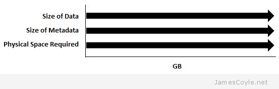
Anyway, back to sparse files. The idea of a sparse file is to remove the need to allocate the full size of the file to a physical disk. I can, for example, create a qcow2 image with a data capacity of 10GB that will take up just several KBs of physical space until data is saved to the qcow2 image. As data is saved to the qcow2 image, the physical space used by the image will increase (the data has to be stored somewhere, right?). In addition, as will the metadata because each new cluster that’s required by the qcow2 file will have it’s own entry in the metadata section of the file.

qemu-img comes with various options for setting the allocation when creating new disk images.

  • preallocation=metadata – allocates the space required by the metadata but doesn’t allocate any space for the data. This is the quickest to provision but the slowest for guest writes.
  • preallocation=falloc –  allocates space for the metadata and data but marks the blocks as unallocated. This will provision slower than metadata but quicker than full. Guest write performance will be much quicker than metadata and similar to full.
  • preallocation=full – allocates space for the metadata and data and will therefore consume all the physical space that you allocate (not sparse). All empty allocated space will be set as a zero. This is the slowest to provision and will give similar guest write performance to falloc.

Example command:

qemu-img create -f qcow2 -o preallocation=falloc image.qcow2 1G

The performance impact here is when the virtual image needs to grow in order to store new information written to it. For each new write a new cluster will need to be provisioned and a metadata index entry referencing the new cluster. Depending on the above option selected, the OS may have to allocate a new sector for both the index and the data cluster incurring a performance penalty. Once the disk has been expanded (e.g. or preallocation=full) then there is no penalty on assigning a new cluster as all the clusters are already assigned and available.

See qcow2 preallocation for some examples and benchmarks of the above attributes.

Encryption

qcow2 images are not encrypted by default, so not using encryption couldn’t be more simple. Of course, your data will not be encrypted (unless you use some other process on top of the virtual storage layer) but you’ll save all those CPU cycles when reading and writing the data.

Compression

qcow2 is, at best, a bit weird when it comes to compression (encryption works the same way, too!) in that compression is a one time event, or process that you run to compress an existing image. Any data written after this will be stored uncompressed.

The next thing is to understand compression itself – compression (under the right circumstances) will reduce the size of the data stored on disk at the expense of CPU to compress (one off) and decompress (every time the data is accessed) the data. In certain circumstances, compression can result in a quicker read for the process consuming the data, such as where CPU is abundant and IO bandwidth is very small.

As always, testing your scenarios is the best way to understand the impact.


dd Cheat Sheet

Get Social!

dd is one of the most versatile IO tools available for Linux. It’s used in a variety of ways ranging from Disk Benchmarking through to creating SWAP files and copying downloaded disk images to physical disks.

dd takes the following common switches:

  • if is the input file name and location.
  • of is the name and location of the output file.
  • bs is the block size that will be used to read and/ or write the file. Increasing this can help with performance  or dictate how much data will be read or written.
  • count is the number of blocks that will be used.
  • seek is the number of blocks on the output file that will be skipped before writing any data.
  • skip is the number of blocks that will be skipped on the input file before starting to read data.
  • conv is a comma separated list of additional parameters that can be used. See the man dd for more information.

The below headings will list a few example uses of dd in a typical Linux environment.

Backup disk partition with dd

You can use dd to copy an entire disk partition to a virtual disk file. This can be useful for creating a backup or to clone the disk to another machine.

dd if=/dev/sda1 of=~/localdisk_sda1.img

You can use this method to read a CD-ROM, USB drive or Flash disk to a file in the same way – just make sure the device is inserted and point the if= part of the dd command to the relevant /dev/ device.

You could also compress the image as part of the process with gzip.

dd if=/dev/sda1 | gzip -c > ~/localdisk_sda1.img.gz

Restore disk partition with dd

Similar to the above command, you can use dd to replace a disk’s partition with a virtual disk file.

dd if=~/localdisk_sda1.img of=/dev/sda1

If you compressed the image then you can decompress it first all in one go:

gunzip -c ~/localdisk_sda1.img.gz | dd of=/dev/sda1

Create a fixed size file with dd

You can create a fixed size file with DD that will be created in the location you specify.

dd if=/dev/zero of=/root/test bs=1024 count=1

This will create a file in /root/test of 1024 bytes in size. Increase either bs or count to change the size of the file. The resulting size will be bs count. You can also use shorhand sizes such as K, M and G with bs, for example bs=1G,

dd if=/dev/zero of=upload_test bs=file_size count=1

Create a SWAP file with dd

dd can be used to create a SWAP file that can be used as a SWAP device by your computer. This is often needed with smaller instances on Cloud providers such as AWS.

The starting point is the same as the above command to create a file with the size that you’d like to use for swap. See my other blog post for more info.

Split a file with dd

dd can be used to read just part of a file, given offset and length coordinates. The below example will skip the first 100 bytes of the file and output the proceeding 10 bytes (byte 101 – 111).

dd if=filetosplit of=partfile bs=1 count=10 skip=100

You could repeat this process to split a large file into multiple smaller files, to be able to email it for example.

dd if=filetosplit of=partfile1 bs=1 count=100
dd if=filetosplit of=partfile2 bs=1 count=100 skip=100
dd if=filetosplit of=partfile3 bs=1 count=100 skip=200

Merge multiple files with dd

You can merge multiple files into a single file with dd. Following on from the above split example, the below will rejoin the 3 file parts into a single file.

dd if=partfile1 of=joinedfile bs=1 count=100
dd if=partfile2 of=joinedfile bs=1 count=100 seek=100
dd if=partfile3 of=joinedfile bs=1 count=100 seek=200

Convert text to lower case with dd

You can use the conv switch with dd to transform ascii text from upper case to lower case and visa-versa. Using lcase and ucase in the conv switch will instruct dd to convert the text as it’s written.

The below example will convert all characters in the filetoconvert.txt. file to lower case.

dd if=filetoconvert.txt of=convertedfile.txt conv=lcase


Simple Bonnie++ Example

Category : How-to

Get Social!

Linux penguin
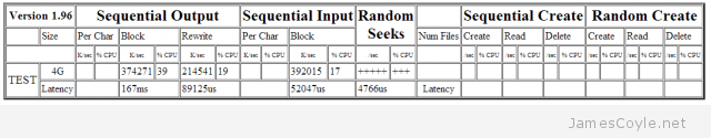
Bonnie++ is a disk and file system benchmarking tool for measuring I/O performance. With Bonnie++ you can quickly and easily produce a meaningful value to represent your current file system performance.

Before using Bonnie++ make sure that you have it installed on your system. In Ubuntu, use apt-get to install the bonnie++ package.

apt-get install bonnie++

Run the bonnie++ command  with the following attributes:

  • [TEST_LOCATION] – is where bonnie++ will create the benchmark operations.
  • [TEST_SIZE] – the size of the test file – this should be greater than double the RAM in your system.
  • [TEST_NAME] – this is simply a label which will be written out with the results.
  • [TEST_USER] – the user who should perform the test. This is not required if you are not running as root.
bonnie++ -d [TEST_LOCATION] -s [TEST_SIZE] -n 0 -m [TEST_NAME] -f -b -u [TEST_USER]

For example:

bonnie++ -d /tmp -s 4G -n 0 -m TEST -f -b -u james

Using uid:1000, gid:1000.
Writing intelligently...done
Rewriting...done
Reading intelligently...done
start 'em...done...done...done...done...done...
Version  1.96       ------Sequential Output------ --Sequential Input- --Random-
Concurrency   1     -Per Chr- --Block-- -Rewrite- -Per Chr- --Block-- --Seeks--
Machine        Size K/sec %CP K/sec %CP K/sec %CP K/sec %CP K/sec %CP  /sec %CP
TEST             4G           374271  39 214541  19           392015  17 +++++ +++
Latency                         167ms   89125us             52047us    4766us

1.96,1.96,TEST,1,1387339401,4G,,,,374271,39,214541,19,,,392015,17,+++++,+++,,,,,,,,,,,,,,,,,,,167ms,89125us,,52047us,4766us,,,,,,

The easiest way to understand the results of a bonnie++ test is to run the output  through the bon_csv2html utility. This perl script uses the bonnie++ results and generates a HTML page which you can later open with your web browser.

Copy the last line of the bonnie++ output into the echo command to replace [RESULTS] and alter the [OUTPUT] path to point to where you would like to save your results.

echo "[RESULTS]" | bon_csv2html > [OUTPUT]

Example command:

echo "1.96,1.96,TEST,1,1387339401,4G,,,,374271,39,214541,19,,,392015,17,+++++,+++,,,,,,,,,,,,,,,,,,,167ms,89125us,,52047us,4766us,,,,,," | bon_csv2html > /tmp/test.html

Finally open the output file with your web browser.

bonnie-results-html

See my other post on using bonnie++ to benchmark your file system.


Benchmark disk IO with DD and Bonnie++

Get Social!

Benchmarking disk or file system IO performance can be tricky at best. The problem is that modern file systems leverage various techniques to ensure that the best performance is achieved such as caching files in RAM. This means that unless you circumvent the disk cache, your reported speeds will be reporting how quickly the files can be read from memory.

In this example, I’ll cover benchmarking a Linux file system using two methods; dd for the easy route, and bonnie++ for a more comprehensive test.

dd

Write

You can use dd to create a large file as quickly as possible to see how long it takes. It’s a very basic test and not very customisable however it will give you a sense of the performance of the file system. You must make sure this file is larger than the amount of RAM you have on your system to avoid the whole file being cached in memory.

It’s usually installed out-of-the-box with most Linux file systems which makes it an ideal tool in locked-down environments or environments where it’s tricky to get packages installed onto. Use the below command substituting [PATH] with the filesystem path to test, [BLOCK_SIZE] with the block size and [LOOPS] for the amount of blocks to write.

time sh -c "dd if=/dev/zero of=[PATH] bs=[BLOCK_SIZE]k count=[LOOPS] && sync"

A break down of the command is as follows:

  • time – times the overall process from start to finish
  • of= this is the path which you would like to test. The path must be read/ writable.
  • bs= is the block size to use. If you have a specific load which you are testing for, make this value mirror the write size which you would expect.
  • sync – forces the process to write the entire file to disk before completing. Note, that dd will return before completing but the time command will not, therefore the time output will include the sync to disk.

The below example uses a 4K block size and loops 2000000 times. The resulting write size will be around 7.6GB.

time sh -c "dd if=/dev/zero of=/mnt/mount1/test.tmp bs=4k count=2000000 && sync"
2000000+0 records in
2000000+0 records out
8192000000 bytes transferred in 159.062003 secs (51501929 bytes/sec)
real 2m41.618s
user 0m0.630s
sys 0m14.998s

Now, let’s do the math. dd tells us how many bytes were written, and the time command tells us how long it took – use the real output at the bottom of the output. Use the formula BYTES / SECONDS. For these larger tests, convert bytes to KB or MB to make more sensible numbers.

(8192000000 / 1024 / 1024) / ((2 * 60) + 41.618)

Bytes converted to MB / (2 minutes + 41.618 seconds)

This gives us an average of 48.34 megabytes per second over the duration of the test.

Read

We can also use dd to test the read speed of a disk by reading the file we created and timing the process. Before we do that, we need to flush the file cache by writing another file which is about the size of the RAM installed on the test system. If we don’t do this, the file we just created will be partially in RAM and therefore the read test will not be completely read from disk.

Create a file using dd which is about the same size as the RAM installed on the system. The below assumes 2GB of RAM is installed. You can check how much RAM is installed with free.

dd if=/dev/zero of=/mnt/mount1/clearcache.tmp bs=4k count=524288

Now for the read test of our original file.

time sh -c "dd if=/mnt/mount1/test.tmp of=/dev/null bs=4k"

And process the time result the same was as when writing.

Bonnie++

Bonnie++ is a small utility with the purpose of benchmarking file system IO performance. It’s commonly available in Linux repositories or available from source from the home page.

On Debian/ Ubuntu based systems, use the apt-get command.

apt-get install bonnie++

Just like with DD, we need to minimise the effect of file caching and therefore the tests should be performed on datasets larger than the amount of RAM you have on the test system. Some people suggest that you should use datasets up to 20 times the amount of RAM, others suggest twice the amount of RAM. Whichever you use, always use the same dataset size for all tests performed to ensure the results are comparable.

There are many commands which can be used with bonnie++, too many to cover here so let’s look at some of the common ones.

  • -d – is used to specify the file system directory to use to benchmark.
  • -u – is used to run a a particular user. This is best used if you run the program as root. This is the UID or the name.
  • -g – is used to run as a particular group. This is the GID or the name.
  • -r – is used to specify the amount of RAM in MB the system has installed. This is total RAM, and not free RAM. Use free -m to find out how much RAM is on your system.
  • -b – removes write buffering and performs a sync at the end of each bonnie++ operation.
  • -s – specifies the dataset size to use for the IO test in MB.
  • -n – is the number of files to use for the create files test.
  • -m – this adds a label to the output so that you can understand what the test was at a later date.
  • -x – is used to repeat the tests n times. Change n to the number of how many times to run the tests.

bonnie++ performs multiple tests, depending on the arguments used, and does not display much until the tests are complete. When the tests complete, two outputs are visible. The bottom line is not readable (unless you really know what you are doing) however above that is a table based output of the results of the tests performed.

Let’s start with a basic test, telling bonnie++ where to test and how much RAM is installed, 2GB in this example. bonnie++ will then use a dataset twice the size of the RAM for tests. As I am running as root, I am specifying a user name.

bonnie++ -d /tmp -r 2048 -u james

bonnie++ will take a few minutes, depending on the speed of your disks and return with something similar to the output below.

Using uid:1000, gid:1000.
Writing a byte at a time...done
Writing intelligently...done
Rewriting...done
Reading a byte at a time...done
Reading intelligently...done
start 'em...done...done...done...done...done...
Create files in sequential order...done.
Stat files in sequential order...done.
Delete files in sequential order...done.
Create files in random order...done.
Stat files in random order...done.
Delete files in random order...done.
Version 1.96 ------Sequential Output------ --Sequential Input- --Random-
Concurrency 1 -Per Chr- --Block-- -Rewrite- -Per Chr- --Block-- --Seeks--
Machine Size K/sec %CP K/sec %CP K/sec %CP K/sec %CP K/sec %CP /sec %CP
ubuntu 4G 786 99 17094 3 15431 3 4662 91 37881 4 548.4 17
Latency 16569us 15704ms 2485ms 51815us 491ms 261ms
Version 1.96 ------Sequential Create------ --------Random Create--------
ubuntu -Create-- --Read--- -Delete-- -Create-- --Read--- -Delete--
 files /sec %CP /sec %CP /sec %CP /sec %CP /sec %CP /sec %CP
 16 142 0 +++++ +++ +++++ +++ +++++ +++ +++++ +++ +++++ +++
Latency 291us 400us 710us 382us 42us 787us
1.96,1.96,ubuntu,1,1378913658,4G,,786,99,17094,3,15431,3,4662,91,37881,4,548.4,17,16,,,,,142,0,+++++,+++,+++++,+++,+++++,+++,+++++,+++,+++++,+++,16569us,15704ms,2485ms,51815us,491ms,261ms,291us,400us,710us,382us,42us,787us

The output shows quite a few statistics, but it’s actually quite straight forward once you understand the format. First, discard the bottom line (or three lines in the above output) as this is the results separated by a comma. Some scripts and graphing applications understand these results but it’s not so easy for humans. The top few lines are just the tests which bonnie++ performs and again, can be discarded.

Of cause, all the output of bonnie++ is useful in some context however we are just going to concentrate on random read/ write, reading a block and writing a block. This boils down to this section:

Version 1.96 ------Sequential Output------ --Sequential Input- --Random-
Concurrency 1 -Per Chr- --Block-- -Rewrite- -Per Chr- --Block-- --Seeks--
Machine Size K/sec %CP K/sec %CP K/sec %CP K/sec %CP K/sec %CP /sec %CP
ubuntu 4G 786 99 17094 3 15431 3 4662 91 37881 4 548.4 17
Latency 16569us 15704ms 2485ms 51815us 491ms 261ms

The above output is not the easiest output to understand due to the character spacing but you should be able to follow it, just. The below points are what we are interested in, for this example, and should give you a basic understanding of what to look for and why.

  • ubuntu is the machine name. If you specified -m some_test_info this would change to some_test_info.
  • 4GB is the total size of the dataset. As we didn’t specify -s, a default of RAM x 2 is used.
  • 17094 shows the speed in KB/s which the dataset was written. This, and the next three points are all sequential reads – that is reading more than one data block.
  • 15431 is the speed at which a file is read and then written and flushed to the disk.
  • 37881 is the speed the dataset is read.
  • 548.4 shows the number of blocks which bonnie++ can seek to per second.
  • Latency number correspond with the above operations – this is the full round-trip time it takes for bonnie++ to perform the operations.

Anything showing multiple +++ is because the test could not be ran with reasonable assurance on the results because they completed too quickly. Increase -n to use more files in the operation and see the results.

bonnie++ can do much more and, even out of the box, show much more but this will give you some basic figures to understand and compare. Remember, always perform tests on datasets larger than the RAM you have installed, multiple times over the day, to reduce the chance of other processes interfering with the results.


Set I/O Priority for Proxmox/ OpenVZ Containers

Category : How-to

Get Social!

proxmox logo gradSince the 2.6.18-028stable021 kernel, it has been possible to set the I/O priority of an OpenVZ container. It is not currently possible to set any I/O limits for containers, only the priority. If you require I/O limits you should use KVM.

The higher the priority is for a container, the more time the container will have for using disks. You can choose between 0 – 7 inclusive, the default value is 4. The higher the value you use, the more I/O time your container will receive. Remember, as this is a priority system each container setting is relative to another. For example, if you set all your containers to priority 7, they will still receive the same amount of I/O time each.

To set the I/O priority of an OpenZV container, login to the host using the console and use the below command.

vzctl set [VM ID] --ioprio [Priority] --save

Replace [VM ID] with the ID of the container you would like to modify, and replace [Priority] with the priority value to use between 0 and 7. The below example sets the priority of container 200 to 7.

vzctl set 200 --ioprio 7 --save

You can also edit the config file directly. In Proxmox this is saved in /etc/pve/openvz/[VMID].conf

Add, or change the existing entry in the conf file to: IOPRIO=”[Priority]”

You will need to reboot the container for the changes to take effect.


Visit our advertisers

Quick Poll

Do you use ZFS on Linux?

Visit our advertisers