Mount NFS volume in a Proxmox OpenVZ container

Mount NFS volume in a Proxmox OpenVZ container

Category : How-to

Get Social!

openvz-logo-150px_new_3There are various options for adding additional storage to an OpenVZ container. You can add additional storage to the containers root volume to simply increase the overall storage available to the container. For external storage, or storage on another disk to the root partition of the container there are bind mounts.

With some light work you can also use NFS mounts inside an OpenVZ container. Before NFS will work in a container a command needs to be ran on the host to enable NFS features in the container.

If you do not enable NFS on the container, you will get the following error:

mount: unknown filesystem type 'nfs'

Open a Terminal on the host machine and run the below command to check that the modules are loaded in the kernel:

modprobe nfs

Then run the below command to enable NFS on the container. Make sure container is turned off or restart the container after issuing the command.

vzctl set 998 --features "nfs:on" --save

This writes a change to the containers config file. To avoid using the command, you could simply edit the config file directly and add the below text to the bottom of the file:

FEATURES="nfs:on"

Start the container and make sure that the required packages are installed.

apt-get install nfs-common

If you do not have the required packages installed you may receive the following error

mount: wrong fs type, bad option, bad superblock on 192.168.50.252:/dspool/compressed,
 missing codepage or helper program, or other error
 (for several filesystems (e.g. nfs, cifs) you might
 need a /sbin/mount.<type> helper program)
 In some cases useful info is found in syslog - try
 dmesg | tail or so

Finally, run the mount command to mount your NFS directory.

mount -t nfs 10.10.10.5:/storage/compressed /mnt/testmount

Proxmox OpenVZ SWAP and Performance

Get Social!

openvz-logo-150px_new_3 I have been having trouble with a Proxmox node which is only running OpenVZ containers however it is at the upper limit of its RAM resources. Over time, I noticed that Proxmox used SWAP (virtual memory, page file, etc), quite aggressively, to make sure there was always some RAM free. That sounds fantastic, and is just what I would expect the Proxmox server to be doing, except it does it all too well. Proxmox made sure that around 40% of the RAM on the host machine was free at the expense of moving many running processes across all the running containers to SWAP. This is how Linux works, by design, and is expected behaviour. Running processes which have memory which hasn’t been touched in a while have their memory moved to SWAP. This allows other applications which need the memory right now to use it and anything left over can be used as cache by the kernel. When a process with memory in SWAP needs to use that memory, it needs to be read from SWAP and back into memory so that it can be used. There is a huge overhead with this process and will often be noticed when you use a container which has not been used in a while – at the start everything will be slow until all the required memory items have been read from SWAP and put back into RAM. To help with this situation we can do two things:

  • Make sure SWAP is always on a fast disk with plenty of free IO bandwidth. On a small installation, this should not be on the same disk as your container file systems. SSDs can also bring a huge performance benefit over conventional mechanical drives.
  • Reduce the amount of RAM which Proxmox keeps free by making the algorithm which moves memory to SWAP less aggressive.

Move SWAP to fast storage

Generally, and when installing Proxmox for the first time a SWAP partition will be created on your hard disk. By default, this will be the same partition as your Proxmox operating system and your container storage. On a slow mechanical disk, this will result in far too much IO concurrency – that is different processes trying to read or write to a disk at the same time – which will massively affect server performance. One thing we can move to another disk is system wide swap.

You can either use a new file, disk, partition or block device for your new swap location. You will then need to turn your old SWAP device off to stop it from being used. Use the below examples to move your SWAP device.

See this post for a quick script to automatically create a SWAP file.

Make a new SWAP device as a file

Create a file on your file system and enable it to be used as a SWAP device. The below example uses the mount /mnt/swapdrive and the file swapfile to use as your new swap device with a size of 4096 MB.

dd if=/dev/zero of=/mnt/swapdrive/swapfile bs=1M count=4096

You will then need to format the file as SWAP with the below command.

mkswap /mnt/swapdrive/swapfile

Make a new SWAP device as a partition

Use the below command to use a drive partition as your new SWAP device. The below example uses /dev/sdc3 as your SWAP partition. You must have precreated this partition for it to be available.

mkswap /dev/sdc3
swapon /dev/sdc3

Turn a new SWAP device on

Once you have a new SWAP device created, either a file or a disk or partition you will need to enable it. Use the swapon command. The below shows an example of a file and disk partition command:

swapon /mnt/swapdrive/swapfile
swapon /dev/sdc3

Turn off the old SWAP device

To turn off the old SWAP device, first identify it using swapon -s.

swapon -s

Then, use the swapoff command to turn the device off. The below example is the default Proxmox SWAP device location.

swapoff /dev/mapper/pve-swap

Clear SWAP space without rebooting

You can clear your SWAP memory by turning the system wide SWAP memory off and then back on again. Run the below commands to turn off your system wide SWAP space forcing all the SWAP to be read back into RAM. You must have enough RAM for available on your system for this to work correctly. Once this has completed, run the second command to turn SWAP back on again. You can also use this to make your SWAP memory changes take effect.

swapoff -a 
swapon -a

Make the SWAP file persist after rebooting

To make sure your SWAP file is mounted the next time your machine reboots you’ll need to add an entry to the fstab file.

Open the fstab file with your text editor:

vi /etc/fstab

And add a line, similar to the below making sure the first attribute is the location of your newly created SWAP file.

/mnt/swapdrive/swapfile  swap  swap  defaults  0  0

Change the ‘swapiness’ setting

To change how aggressively Proxmox, or other Linux distribution, moves process memory to SWAP we have a swapiness attribute. The swapiness setting is a kernel setting which is permanently set in the /etc/sysctl.conf file, or temporarily using sysctl.

The swapiness setting takes a value between 0 and 100. Using 0 will virtually turn off using SWAP, except to avoid an out of memory exception (oom). Using a value of 100 will cause the system to use SWAP as often as possible and will likely degrade system performance servilely. A value of 60 is the default for Proxmox.

Change the swapiness value for the current boot

To change your swapiness value for the current boot, use the below command. The value will be reset after rebooting. The following example will set the swapiness value to 20.

sysctl -w vm.swappiness=20

Permanently change the swapiness value

Use the below command to permanently change your swapiness value. Note that this will not affect the current boot.

vi  /etc/sysctl.conf

And add the following to give a swapiness of 20

vm.swappiness=20

Benchmark disk IO with DD and Bonnie++

Get Social!

Benchmarking disk or file system IO performance can be tricky at best. The problem is that modern file systems leverage various techniques to ensure that the best performance is achieved such as caching files in RAM. This means that unless you circumvent the disk cache, your reported speeds will be reporting how quickly the files can be read from memory.

In this example, I’ll cover benchmarking a Linux file system using two methods; dd for the easy route, and bonnie++ for a more comprehensive test.

dd

Write

You can use dd to create a large file as quickly as possible to see how long it takes. It’s a very basic test and not very customisable however it will give you a sense of the performance of the file system. You must make sure this file is larger than the amount of RAM you have on your system to avoid the whole file being cached in memory.

It’s usually installed out-of-the-box with most Linux file systems which makes it an ideal tool in locked-down environments or environments where it’s tricky to get packages installed onto. Use the below command substituting [PATH] with the filesystem path to test, [BLOCK_SIZE] with the block size and [LOOPS] for the amount of blocks to write.

time sh -c "dd if=/dev/zero of=[PATH] bs=[BLOCK_SIZE]k count=[LOOPS] && sync"

A break down of the command is as follows:

  • time – times the overall process from start to finish
  • of= this is the path which you would like to test. The path must be read/ writable.
  • bs= is the block size to use. If you have a specific load which you are testing for, make this value mirror the write size which you would expect.
  • sync – forces the process to write the entire file to disk before completing. Note, that dd will return before completing but the time command will not, therefore the time output will include the sync to disk.

The below example uses a 4K block size and loops 2000000 times. The resulting write size will be around 7.6GB.

time sh -c "dd if=/dev/zero of=/mnt/mount1/test.tmp bs=4k count=2000000 && sync"
2000000+0 records in
2000000+0 records out
8192000000 bytes transferred in 159.062003 secs (51501929 bytes/sec)
real 2m41.618s
user 0m0.630s
sys 0m14.998s

Now, let’s do the math. dd tells us how many bytes were written, and the time command tells us how long it took – use the real output at the bottom of the output. Use the formula BYTES / SECONDS. For these larger tests, convert bytes to KB or MB to make more sensible numbers.

(8192000000 / 1024 / 1024) / ((2 * 60) + 41.618)

Bytes converted to MB / (2 minutes + 41.618 seconds)

This gives us an average of 48.34 megabytes per second over the duration of the test.

Read

We can also use dd to test the read speed of a disk by reading the file we created and timing the process. Before we do that, we need to flush the file cache by writing another file which is about the size of the RAM installed on the test system. If we don’t do this, the file we just created will be partially in RAM and therefore the read test will not be completely read from disk.

Create a file using dd which is about the same size as the RAM installed on the system. The below assumes 2GB of RAM is installed. You can check how much RAM is installed with free.

dd if=/dev/zero of=/mnt/mount1/clearcache.tmp bs=4k count=524288

Now for the read test of our original file.

time sh -c "dd if=/mnt/mount1/test.tmp of=/dev/null bs=4k"

And process the time result the same was as when writing.

Bonnie++

Bonnie++ is a small utility with the purpose of benchmarking file system IO performance. It’s commonly available in Linux repositories or available from source from the home page.

On Debian/ Ubuntu based systems, use the apt-get command.

apt-get install bonnie++

Just like with DD, we need to minimise the effect of file caching and therefore the tests should be performed on datasets larger than the amount of RAM you have on the test system. Some people suggest that you should use datasets up to 20 times the amount of RAM, others suggest twice the amount of RAM. Whichever you use, always use the same dataset size for all tests performed to ensure the results are comparable.

There are many commands which can be used with bonnie++, too many to cover here so let’s look at some of the common ones.

  • -d – is used to specify the file system directory to use to benchmark.
  • -u – is used to run a a particular user. This is best used if you run the program as root. This is the UID or the name.
  • -g – is used to run as a particular group. This is the GID or the name.
  • -r – is used to specify the amount of RAM in MB the system has installed. This is total RAM, and not free RAM. Use free -m to find out how much RAM is on your system.
  • -b – removes write buffering and performs a sync at the end of each bonnie++ operation.
  • -s – specifies the dataset size to use for the IO test in MB.
  • -n – is the number of files to use for the create files test.
  • -m – this adds a label to the output so that you can understand what the test was at a later date.
  • -x – is used to repeat the tests n times. Change n to the number of how many times to run the tests.

bonnie++ performs multiple tests, depending on the arguments used, and does not display much until the tests are complete. When the tests complete, two outputs are visible. The bottom line is not readable (unless you really know what you are doing) however above that is a table based output of the results of the tests performed.

Let’s start with a basic test, telling bonnie++ where to test and how much RAM is installed, 2GB in this example. bonnie++ will then use a dataset twice the size of the RAM for tests. As I am running as root, I am specifying a user name.

bonnie++ -d /tmp -r 2048 -u james

bonnie++ will take a few minutes, depending on the speed of your disks and return with something similar to the output below.

Using uid:1000, gid:1000.
Writing a byte at a time...done
Writing intelligently...done
Rewriting...done
Reading a byte at a time...done
Reading intelligently...done
start 'em...done...done...done...done...done...
Create files in sequential order...done.
Stat files in sequential order...done.
Delete files in sequential order...done.
Create files in random order...done.
Stat files in random order...done.
Delete files in random order...done.
Version 1.96 ------Sequential Output------ --Sequential Input- --Random-
Concurrency 1 -Per Chr- --Block-- -Rewrite- -Per Chr- --Block-- --Seeks--
Machine Size K/sec %CP K/sec %CP K/sec %CP K/sec %CP K/sec %CP /sec %CP
ubuntu 4G 786 99 17094 3 15431 3 4662 91 37881 4 548.4 17
Latency 16569us 15704ms 2485ms 51815us 491ms 261ms
Version 1.96 ------Sequential Create------ --------Random Create--------
ubuntu -Create-- --Read--- -Delete-- -Create-- --Read--- -Delete--
 files /sec %CP /sec %CP /sec %CP /sec %CP /sec %CP /sec %CP
 16 142 0 +++++ +++ +++++ +++ +++++ +++ +++++ +++ +++++ +++
Latency 291us 400us 710us 382us 42us 787us
1.96,1.96,ubuntu,1,1378913658,4G,,786,99,17094,3,15431,3,4662,91,37881,4,548.4,17,16,,,,,142,0,+++++,+++,+++++,+++,+++++,+++,+++++,+++,+++++,+++,16569us,15704ms,2485ms,51815us,491ms,261ms,291us,400us,710us,382us,42us,787us

The output shows quite a few statistics, but it’s actually quite straight forward once you understand the format. First, discard the bottom line (or three lines in the above output) as this is the results separated by a comma. Some scripts and graphing applications understand these results but it’s not so easy for humans. The top few lines are just the tests which bonnie++ performs and again, can be discarded.

Of cause, all the output of bonnie++ is useful in some context however we are just going to concentrate on random read/ write, reading a block and writing a block. This boils down to this section:

Version 1.96 ------Sequential Output------ --Sequential Input- --Random-
Concurrency 1 -Per Chr- --Block-- -Rewrite- -Per Chr- --Block-- --Seeks--
Machine Size K/sec %CP K/sec %CP K/sec %CP K/sec %CP K/sec %CP /sec %CP
ubuntu 4G 786 99 17094 3 15431 3 4662 91 37881 4 548.4 17
Latency 16569us 15704ms 2485ms 51815us 491ms 261ms

The above output is not the easiest output to understand due to the character spacing but you should be able to follow it, just. The below points are what we are interested in, for this example, and should give you a basic understanding of what to look for and why.

  • ubuntu is the machine name. If you specified -m some_test_info this would change to some_test_info.
  • 4GB is the total size of the dataset. As we didn’t specify -s, a default of RAM x 2 is used.
  • 17094 shows the speed in KB/s which the dataset was written. This, and the next three points are all sequential reads – that is reading more than one data block.
  • 15431 is the speed at which a file is read and then written and flushed to the disk.
  • 37881 is the speed the dataset is read.
  • 548.4 shows the number of blocks which bonnie++ can seek to per second.
  • Latency number correspond with the above operations – this is the full round-trip time it takes for bonnie++ to perform the operations.

Anything showing multiple +++ is because the test could not be ran with reasonable assurance on the results because they completed too quickly. Increase -n to use more files in the operation and see the results.

bonnie++ can do much more and, even out of the box, show much more but this will give you some basic figures to understand and compare. Remember, always perform tests on datasets larger than the RAM you have installed, multiple times over the day, to reduce the chance of other processes interfering with the results.


Create a ZFS volume on Ubuntu

Category : How-to

Get Social!

zfs-linuxZFS is a disk and logical volume manager combining raid like functionality with guaranteeing data integrity. Every block of data read by ZFS is checksumed and recovered if an error is found. ZFS also periodically checks the entire file system for any silent corruption which may have occurred since the data was written.

ZFS was initially developed by Sun for use in Solaris and as such was not available on Linux distributions. Thanks to some clever guys over at ZFS on Linux, this has now changed. We can now install the ZFS on most Linux distributions such as Debain/ Ubuntu and Red Hat/ CentOS.

ZFS provides a data volume which can have multiple mount points, spanning multiple disks. Disks can be combined into virtual groups to allow for various redundancy options:

  • Mirror – data will be mirrored across disks, equivalent to RAID 1. This is quite simply a copy of one disk to another every time data is changed. You require a minimum of two disks for a mirrored set. This provides the best redundancy but requires the most space. For example, if you use 2x 500GB disks, only 500GB will be available as the other 500GB will be a copy of the first disk.
  • Stripe – data will be stored across all available disks, equivalent to RAID 0. In a two disk striped array, half of a file would be on disk one and half of the file on disk two. This provides the fastest read and write speeds but it offers no redundancy. In the event of a failed disk, all data on the stripe will be lost.
  • RAID-Z – data will be written to all but one of the disks, with the remaining disk used for parity. This is equivalent to RAID 5. A minimum of three disks are required with one disk always being used for parity. In the even of a single disk failure, all data can be recovered and in fact, will still be accessible providing no further disks fail. In the even of a second disk failure, all data on the RAIDZ will be lost.
  • RAID-Z 2 and RAID-Z 3 – these are the same as RAIDZ but with two and three disks used for parity respectively. RAID-Z 3 is recommended for highly critical data consistency environments. RAIDZ-2 requires a minimum of 4 disks, and RAID-Z 3 requires 5 disks as a minimum.

zfs highlevel structure diagram

In addition to these virtual groups, multiple groups can be combined. For example, you can mirror a striped virtual volume to create a RAID 10. This gives the added performance of striped volumes with the redundancy of mirrored volumes.

For our below example, we are going to create a single RAIDZ 1 with three disks. This gives us two full disks of storage, and a further disk for parity.

Installing ZFS on Ubuntu

Before we can start using ZFS, we need to install it. Simply add the repository to apt-get with the following command:

apt-add-repository --yes ppa:zfs-native/stable

In a minimum package install, you may not have the apt-add-repository installed.

The program 'apt-add-repository' is currently not installed.  You can install it by typing:
apt-get install python-software-properties

If this is the case, install it before running the apt-add-repository command.

apt-get install python-software-properties

Update the apt cache with the update argument

apt-get update

Install the ZFS binaries, tools and kernel modules. This may take a while due to the amount of packages apt will have to download, building the tools and the ZFS modules for the kernel.

apt-get install ubuntu-zfs

At this point, it is best to test the kernel was correctly compiled and loaded.

dmesg | grep ZFS

The output should look like below. If it does not try running modprobe zfs.

[  824.725076] ZFS: Loaded module v0.6.1-rc14, ZFS pool version 5000, ZFS filesystem version 5

Create RAID-Z 1 3 disk array

Once ZFS is installed, we can create a virtual volume of our three disks. The three disks should all be the same size, if they are not the smallest disk’s size will be used on all three disks.

Identify the disks you would like to use with fdisk. Some disk controllers may have their own naming conventions and administration tools but we’ll use fdisk in this example. Whilst we are on this point, raid controllers should not be set up with raid functionality when using ZFS. Some of the mechanisms in ZFS can be fooled with an underlying layer also doing data parity and therefore data corruption can occur in this environment.

fdisk -l | grep /dev/

The output will look like:

Disk /dev/vdb doesn't contain a valid partition table
Disk /dev/vdc doesn't contain a valid partition table
Disk /dev/vdd doesn't contain a valid partition table

And there we have it! The three disks to add to our ZFS array. Note, I have removed the root volume in this example to avoid confusion.

Run the zpool create command passing in the disks to use for the array as arguments. By specifying the argument -f it removes the need to create partitions on the disks prior to creating the array. This command creates a zpool called datastore however you can change this to suit your needs.

zpool create -f datastore raidz /dev/vdb /dev/vdc /dev/vdd

Confirm the zpool has been created with:

zpool status datastore

The output should be similar to:

  pool: datastore
 state: ONLINE
  scan: none requested
config:

        NAME        STATE     READ WRITE CKSUM
        datastore   ONLINE       0     0     0
          raidz1-0  ONLINE       0     0     0
            vdb1    ONLINE       0     0     0
            vdc1    ONLINE       0     0     0
            vdd1    ONLINE       0     0     0

errors: No known data errors

Create ZFS dataset

At this point, we now have a zpool spanning three disks. One of these is used for parity, giving us the chance to recover in the event of a single disk failure. The next step is to make the volume usable and add features such as compression, encryption or de-duplication.

Multiple datasets or mount points can be created on a single volume. Generally, you do not specify these size of these. Put simply, the storage of the zpool with be available to any dataset as it requires it. You can set up quotas to manage dataset sizes but that won’t be covered in this tutorial.

What we are interested in is creating three volumes; binaries, homes and backups. These will be mounted at /mnt/binaries, /mnt/homes and /mnt/backups respectively. Using zfs create command, create the three required volumes.

We specify the mount point, zpool and dataset name in the command.

zfs create -o mountpoint=[MOUNT POINT] [ZPOOL NAME]/[DATASET NAME]

Example:

zfs create -o mountpoint=/mnt/binaries datastore/binaries
zfs create -o mountpoint=/mnt/homes datastore/homes
zfs create -o mountpoint=/mnt/backups datastore/backups

Test the datasets have been created with zfs list.

zfs list
NAME                 USED  AVAIL  REFER  MOUNTPOINT
datastore            312K  62.6G  38.6K  /datastore
datastore/backups   38.6K  62.6G  38.6K  /mnt/backups
datastore/binaries  38.6K  62.6G  38.6K  /mnt/binaries
datastore/homes     38.6K  62.6G  38.6K  /mnt/homes

And an ls in /mnt should give us the mount points.

ls /mnt/
backups/   binaries/   homes/

You can now use your mounted datasets as required. You can export them as NFS, CIFS or simply use them as local storage!

See my other posts for compression and encryption. Please note, encryption is not currently available on ZFS for Linux.


GlusterFS firewall rules

Category : How-to

Get Social!

gluster-orange-ant
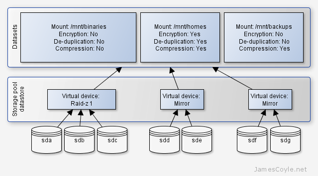
If you can, your storage servers should be in a secure zone in your network removing the need to firewall each machine. Inspecting packets incurs an overhead, not something you need on a high performance file server so you should not run a file server in an insecure zone. If you are using GlusterFS behind a firewall you will need to allow several ports for GlusterFS to communicate with clients and other servers. The following ports are all TCP:

Note: the brick ports have changed since version 3.4. 

  • 24007 – Gluster Daemon
  • 24008 – Management
  • 24009 and greater (GlusterFS versions less than 3.4) OR
  • 49152 (GlusterFS versions 3.4 and later) – Each brick for every volume on your host requires it’s own port. For every new brick, one new port will be used starting at 24009 for GlusterFS versions below 3.4 and 49152 for version 3.4 and above. If you have one volume with two bricks, you will need to open 24009 – 24010 (or 49152 – 49153).
  • 38465 – 38467 – this is required if you by the Gluster NFS service.

The following ports are TCP and UDP:

  • 111 – portmapper

Share GlusterFS volume to a single IP address

Category : How-to

Get Social!

gluster-orange-antWhen you create a new GlusterFS Volume it is publicly available for any server on the network to read.

File servers do not generally have firewalls as they are hosted in a secure zone of a private network. Just because it’s secure doesn’t mean you should leave it wide open for anyone with access to connect to.

Using the auth.allow and auth.reject arguments in GlusterFS we can choose which IP addresses can access the volume. Access is provided at volume level, therefore you will need to alter access permissions on every new volume you create.

Run the below command on each server changing [VOLUME] to match the volume to be accessed and [IP ADDRESS] to be an IP address of the server which can connect to the current server.

gluster volume set [VOLUME] auth.allow [IP ADDRESS]

[IP ADDRESS] does not have to be a single IP address. You can also use an asterisk [*] as a wildcard, or multiple addresses separated by a comma [,]. The below example allows only servers with an IP address on the 10.1.1.x range, and 10.5.5.1 to access volume datastore.. All other servers will be denied access to the volume.

gluster volume set datastore auth.allow 10.1.1.*,10.5.5.1

Visit our advertisers

Quick Poll

How often do you change the password for the computer(s) you use?

Visit our advertisers